Lecture 2 - The architecture of ProtoPNet and its Python implementation
Introduction
In the previous lecture, we covered how to run and debug a simplified learning version of ProtoPNet. This session will focus on the architecture of ProtoPNet and its Python implementation.
When introducing the python implementation in the following, the reader can open main.ipynb, use Ctrl+f to open the search box, fill in the names of the functions or parameters, and then search for the location of the code to be explained.
The main architecture and its python implementation of ProtoPNet
The original Figure 2 in reference [1] describes the schematic diagram of the architecture of ProtoPNet. Here, the original figure is copied to Figure 1 below for readers’ retrieval and comparison.
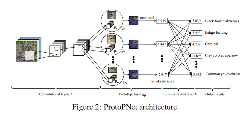
Figure 1 Architecture of ProtoPNet
A description of this architecture is given in Section 2.1 of reference [1], which is restated below:
…… Our network consists of a regular convolutional neural network \(f\), whose parameters are collectively denoted by \({w_{conv}}\), followed by a prototype layer \({g_P}\) and a fully connected layer \(h\) with weight matrix \(w_h\) and no bias. For the regular convolutional network \(f\), our model use the convolutional layers from models such as …, VCG-19, … (initialized with filters pretrained on ImageNet), followed by two additional 1x1 convolutional layers in our experiments. We use ReLU as the activation function for all convolutional layers except the last for which we use the sigmoid activation function……
The above description corresponds to the implementation of each network layer in the following functions of the PPNet class defined in the eighth cell of main.ipynb (see Figure 2).
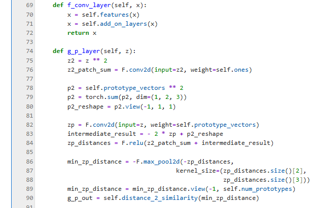

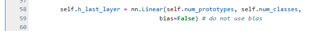
Figure 2. Implementation of network layers in PPNet
where,
self.f_conv_layers functions correspond to convolutional layer \({f}\)
self.g_p_layer function corresponds to the Prototype \(g_p\) layer
self.h_last_layer corresponds to the fully connected layer \(h\) layer
The following sections explain each layer and its corresponding code implementation.
self.f_conv_layers() and its self.features()
Chapter 2.1 of reference [1] describes the following:
……For the regular convolutional network , our model use the convolutional layers from models such as …, VCG-19……
This section corresponds to the self.features in the self.f_conv_layer() function of main.ipynb; it is created in the function named ‘construct_PPNet()’ by ‘features = vgg19_features()’ (as shown in Figure 3).
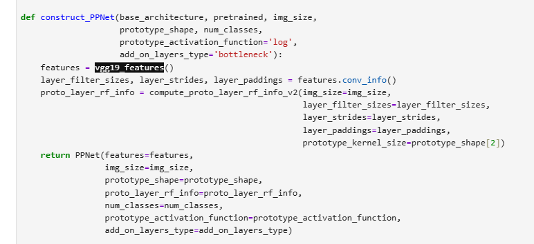
Figure 3 vgg19_features creates features
In the vgg19_features() function, the VGG19 model is constructed by calling VGG_features (cfg) (see Figure 4).
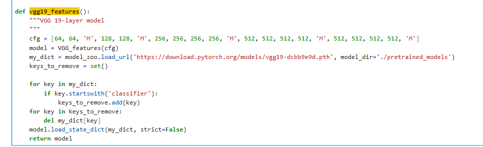
Figure 4 The VGG19 is actually created by VGG_feature(cfg)
The configuration file contains the following entries: cfg=[64,64, ‘M’, 128,128, ‘M’, 256,256,256,256, ‘M’, 512,512,512,512, ‘M’, 512,512,512,512, ‘M’]. The numerical values (e.g., 64,128,256,512, denoted as v) and the letter ‘M’ can be interpreted using the ‘VGG_features._make_layers()’ function (as shown in Figure 5):
M refers to the nn.MaxPool2d with kernel size =2, stride =2, and padding =0;
Each number corresponds to an “output channel of v, kernel size=3, stride=1, padding=1” nn.conv2d and nn.ReLU.
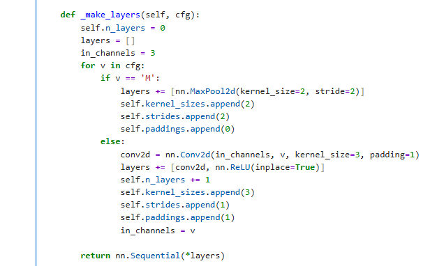
Figure 5 VGG_features._make_layers() function
self.f_conv_layers and its self.add_on_layers()
Reference [1] also has a description of the two additional layers in section 2.1:
……followed by two additional 1 \(\times\) 1 convolutional layers in our experiments. We use ReLU as the activation function for all convolutional layers except the last for which we use the sigmoid activation function……
In main.ipynb, the implementation of these two additional layers is in the 45th line of code in the eighth cell (see Figure 6):
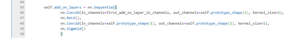
Figure 6 self.add_on_layers
self.g_p_layer
The function description of the prototype layer(\(g_p\)) in paragraph 2.1 of reference [1] is as follows:
…… Given a convolutional output \(z=f(x)\), the \(j\)-th prototype unit \(g_{p_j}\) in the prototype layer \(g_p\) computes the squared \(L^2\) distances between the \(j\)-th prototype \(p_j\) and all patches of \(z\) that have the same shape as \(p_j\), and inverts the distances into similarity scores. The result is an activation map of similarity scores whose value indicates how strong a prototypical part is presented in the image. ….. The activation map of similarity scores produced by each prototype unit \(g_{p_j}\) is then reduced using global max pooling to a single similarity score, which can be understood as how strongly a prototypical part is presented in some patch of the input image……
The corresponding code implementation is in the function ‘g_p_layer (self, z)’ in the 8th cell of main.ipynb, at the about 74th line (figure-7).

Figure 7 g_p_layer(self, z) function
To understand this ‘g_p_layer(self, z)’ function, we need to continue to another description in Section 2.1, paragraph 2 of reference [1]:
……Mathematically, the prototype unit \(g_{p_j}\) computes \(g_{p_j}(z)=\max_{\tilde{z}\in patches(z)} \log{\frac{\|tilde{z}-p_j\|_2^2 + 1}{\| \tilde{z}-p_j \|_2^2+\epsilon}}\) ……
where, \(\| \tilde{z}-p_j \|_2^2 = \| \tilde{z} \|_2^2 + \| p_j \|_2^2 - 2(\tilde{z} \cdot p_j), \tilde{z} \in patches(z)\). Here, \(\| \tilde{z} \|_2^2\) is calculated once for all by means of the 76th line (i.e., z2_patch_sum=F.conv2d(input=z2, weight=self.ones)).
\(\| p_j \|_2^2,j=1,2,...,m\) is obtained by line 78, 79 and 80.
\((\tilde{z} \cdot p_j)\) is obtained by a tricky calculation of an F.conv2d in line 82.
Finally, the sum \(\| \tilde{z} - p_j \|_2^2\), where \(\tilde{z} \in patches(z), j=1,2,...,m\) in line 83 and 84 is obtained.
Note: Here the shape of zp_distance is #batch_size * M * I * J, where I * J is the number of all patches i patches(z).
Lines 86-90 are the exact calculations. Since we’re dealing with a monotonic decreasing function, the calculation can be split into two steps:
self.h_last_layer
The Fully connected layer is described at the beginning and end of paragraph 2.1 in reference [1]:
…… followed by a prototype layer \(g_p\) and a fully connected layer \(h\) with weight matrix \(w_h\) and no bias….
…… Finally, the m similarity scores produced by the prototype layer \(g_p\) are multiplied by the weight matrix \(w_h\) in the fully connected layer \(h\) to produce the output logits, which are normalized using softmax to yield the predicted probabilities for a given image belonging to various classes. …..
Its corresponding implementation is defined in approximately line 58 of main.ipynb eighth cell (see Figure 8):

Figure 8 self.h_last_layer
self.forward()
Finally, self.conv_layers, self.g_p_layer and self.h_last_layer are connected in chain in the self.forward() function of PPNet (Figure 9)
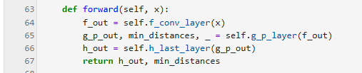
Figure 9 forward function
Summary
This lecture explains how the architecture of PPNet (Figure 2 in the original paper) corresponds to its implementation in main.ipynb. The next lecture will cover the training details of PPNet.