第二讲-ProtoPNet的架构和它的python实现
简介
上一讲已经介绍了如何运行和调试ProtoPNet的简明学习版本。本讲将主要介绍ProtoPNet的架构和它的python实现。
在下文介绍代码的时候,读者可以打开main.ipynb,使用Ctrl+f打开搜索框,填入代码的函数或参数等,就可以搜索得到待讲解的代码的位置。
ProtoPNet的主体架构和代码实现
参考文献[1]的原图2描述了ProtoPNet的架构的示意图,这里把原图复制到下图 1,方便读者检索和对比。
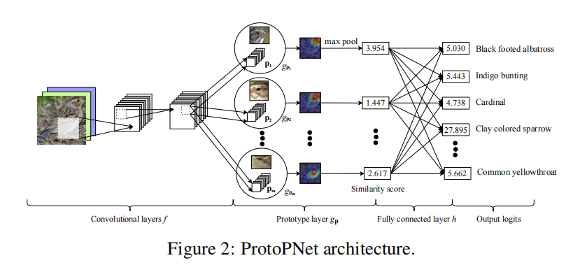
图 1 ProtoPNet的架构
参考文献[1]的2.1章节对该架构有一段描述, 这里复述如下:
…… Our network consists of a regular convolutional neural network \(f\), whose parameters are collectively denoted by \({w_{conv}}\), followed by a prototype layer \({g_P}\) and a fully connected layer \(h\) with weight matrix \(w_h\) and no bias. For the regular convolutional network \(f\), our model use the convolutional layers from models such as …, VCG-19, … (initialized with filters pretrained on ImageNet), followed by two additional 1x1 convolutional layers in our experiments. We use ReLU as the activation function for all convolutional layers except the last for which we use the sigmoid activation function……
以上的描述对应于main.ipynb中的第八个单元中定义的PPNet类的如下函数(如图 2)中的各个network layer的实现。
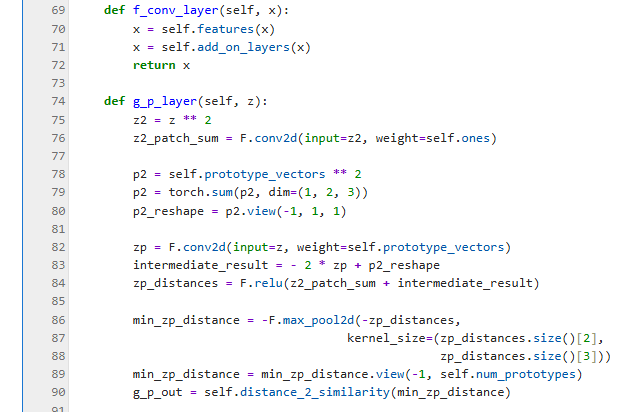

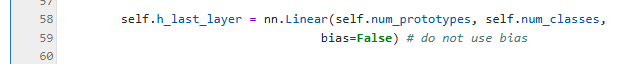
图 2 PPNet中的network layers的实现
其中,
self.f_conv_layers函数对应于Convolutional layers \(f\)
self.g_p_layer函数对应于Prototype layer \(g_p\)
self.h_last_layer对应于Fully connected layer \(h\)
下面分别详细讲解各个layers和对应的代码实现。
self.f_conv_layers()和它的self.features()
参考文献[1]的第2.1章节有下面的一段描述:
……For the regular convolutional network , our model use the convolutional layers from models such as …, VCG-19……
这一段描述对应于main.ipynb中的self.f_conv_layer()函数中的self.features;它是在函数construct_PPNet()中,由’features =vgg19_features()’创建(如图 3)。
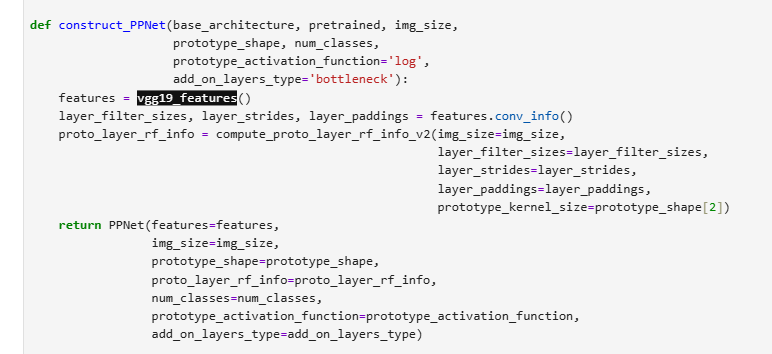
图 3 vgg19_features创建features
在vgg19_features()函数中,VGG19这个模型具体通过类VGG_features(cfg)来构造(如图 4)。
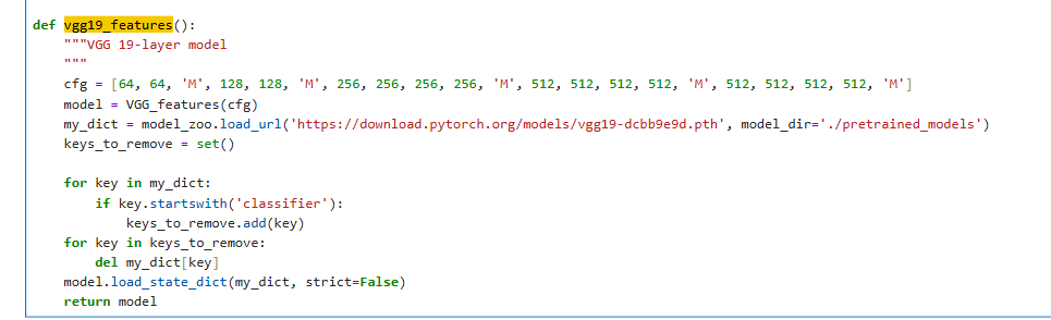
图 4 vgg19实际由VGG_feature(cfg)创建
其中,cfg=[64, 64, ‘M’, 128, 128, ‘M’, 256, 256, 256, 256, ‘M’, 512, 512, 512, 512, ‘M’, 512, 512, 512, 512, ‘M’]。其中的数字(如64, 128, 256, 512, 记为v)和字母’M’的含义,可以结合VGG_features._make_layers()函数(如图 5)来理解:
M是指具有kernel_size=2, stride=2, padding=0的nn.MaxPool2d;
每一个数字对应于一个”输出通道为v, kernel_size=3, stride=1, padding=1”的nn.conv2d和nn.ReLU.
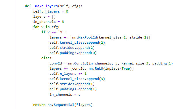
图 5 VGG_features._make_layers()函数
self.f_conv_layers和它的self.add_on_layers()
参考文献[1]的第2.1章节也有一段关于两个additional layer的描述:
……followed by two additional 1 \(\times\) 1 convolutional layers in our experiments. We use ReLU as the activation function for all convolutional layers except the last for which we use the sigmoid activation function……
在main.ipynb中,这两个additional layers的实现在第八个单元的第约45行代码(如图 6):
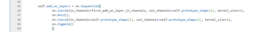
图 6 self.add_on_layers
self.g_p_layer
参考文献[1]的第2.1章节的第2段对prototype layer ()的功能描述如下:
…… Given a convolutional output \(z=f(x)\), the \(j\)-th prototype unit \(g_{p_j}\) in the prototype layer \(g_p\) computes the squared \(L^2\) distances between the \(j\)-th prototype \(p_j\) and all patches of \(z\) that have the same shape as \(p_j\), and inverts the distances into similarity scores. The result is an activation map of similarity scores whose value indicates how strong a prototypical part is presented in the image. ….. The activation map of similarity scores produced by each prototype unit \(g_{p_j}\) is then reduced using global max pooling to a single similarity score, which can be understood as how strongly a prototypical part is presented in some patch of the input image……
相应的代码的实现,在main.ipynb的第八个单元的约74行的函数g_p_layer(self, z)函数。

图 7 g_p_layer(self, z)函数
要理解这个g_p_layer(self, z)函数,还要继续结合参考文献[1]的第2.1章节的第2段的另一段描述:
……Mathematically, the prototype unit \(g_{p_j}\) computes \(g_{p_j}(z)=\max_{\tilde{z}\in patches(z)} \log{\frac{\|tilde{z}-p_j\|_2^2 + 1}{\| tilde{z}-p_j \|_2^2+\epsilon}}\) ……
其中, \(\| \tilde{z}-p_j \|_2^2 = \| \tilde{z} \|_2^2 + \| p_j \|_2^2 - 2(\tilde{z} \cdot p_j), \tilde{z} \in patches(z)\). 这里, \(\| \tilde{z} \|_2^2\) 是通过第76行(z2_patch_sum=F.conv2d(input=z2, weight=self.ones))巧妙地对所有的都一次计算出来。
\(\| p_j \|_2^2,j=1,2,...,m\) 是通过第78、79和80行获得。
\((\tilde{z} \cdot p_j)\) 是由第82行巧妙地通过一个F.conv2d计算获得。
最后由第83、84行的求和得到所有 \(\| \tilde{z} - p_j \|_2^2\), 其中 \(\tilde{z} \in patches(z), j=1,2,...,m\)
注意:这里zp_distances的shape是#batch_size * M * I * J, I和J是 \(\tilde{z}\) 的维度,也就是I*J是 \(patches(z)\) 中的所有patch的数目。
第86-90行是实际计算 \(g_{p_j}(z)=\max_{\tilde{z}\in patches(z)} \log{\frac{\|tilde{z}-p_j\|_2^2 + 1}{\| tilde{z}-p_j \|_2^2+\epsilon}}\)。考虑到 \(g_{p_j}(z)\) 是关于 \(\| \tilde{z} - p_j \|_2^2\) 的单调递减函数,所以 \(g_{p_j}(z)\) 的计算可以变换为两步:
self.h_last_layer
参考文献[1]的第2.1章节的第2段的开始和末尾描述了Fully connected layer \(h\):
…… followed by a prototype layer \(g_p\) and a fully connected layer \(h\) with weight matrix \(w_h\) and no bias….
…… Finally, the m similarity scores produced by the prototype layer \(g_p\) are multiplied by the weight matrix \(w_h\) in the fully connected layer \(h\) to produce the output logits, which are normalized using softmax to yield the predicted probabilities for a given image belonging to various classes. …..
它的对应的实现在main.ipynb的第八单元的约第58行定义(如图 8):

图 8 self.h_last_layer
self.forward()
最后,self.conv_layers、self.g_p_layer和self.h_last_layer在PPNet的self.forward()函数中依次串接起来(如图 9)
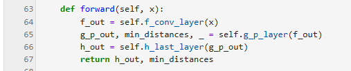
图 9 forward函数
总结
本讲主要讲解了PPNet的架构(原论文的原图2)如何对应于main.ipynb中的实现。下一讲将介绍PPNet的训练细节。