Lecture 1 - How to Run and Debug a student version of ProtoPNet in Jupyterhub

Introduction

This article introduces a simplified student version of the original open-source repository ProtoPNet. The ProtoPNet repository, originally provided by the authors of the paper “This Looks Like That: Deep Learning for Interpretable Image Recognition,” offers a Python implementation of ProtoPNet. However, the paper recommends hardware configurations of 4 NVIDIA Tesla P-100 GPUs or 8 NVIDIA Tesla K-80 GPUs to run the repository. For students or young researchers to ML/AI, however, these hardware requirements can be too demanding.

This concise student version of the original repository is designed to help newcomers in the ML/AI field grasp the AI algorithms easily. The simplified code can be run and debugged on pure CPU environments, allowing readers to meticulously compare and cross-verify each line of code with the algorithm descriptions from the original paper. This process enables readers to master algorithmic principles thoroughly, laying a solid foundation for future rapid migration to GPU environments.

This article is the first lecture on this topic: Learning the ProtoPNet.

Running and debugging of the student version of ProtoPNet in AcdEvent’s Jupyterhub

Interested readers can visit the Academic Simulation Hub and leave a comment at the bottom of the page saying “I want to learn ProtoPNet”. After confirmation, you will receive a free login account and password.

Readers who have obtained the account and password can continue to access Acdevent’s Jupyterhub, to log on to Academic Simulation Hub (Figure 1).

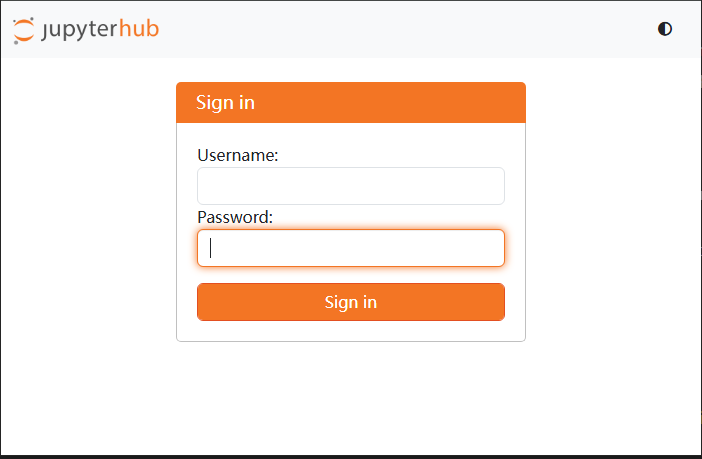
Figure 1 Login to Academic Simulation Hub

After successfully logging into the Academic Simulation Hub, you will see the login interface of the ProtoPNet Simplified student version as shown in Figure 2. The left side is the workspace, and the right side is the Launcher (currently not in use). Under the workspace is a directory named codes.

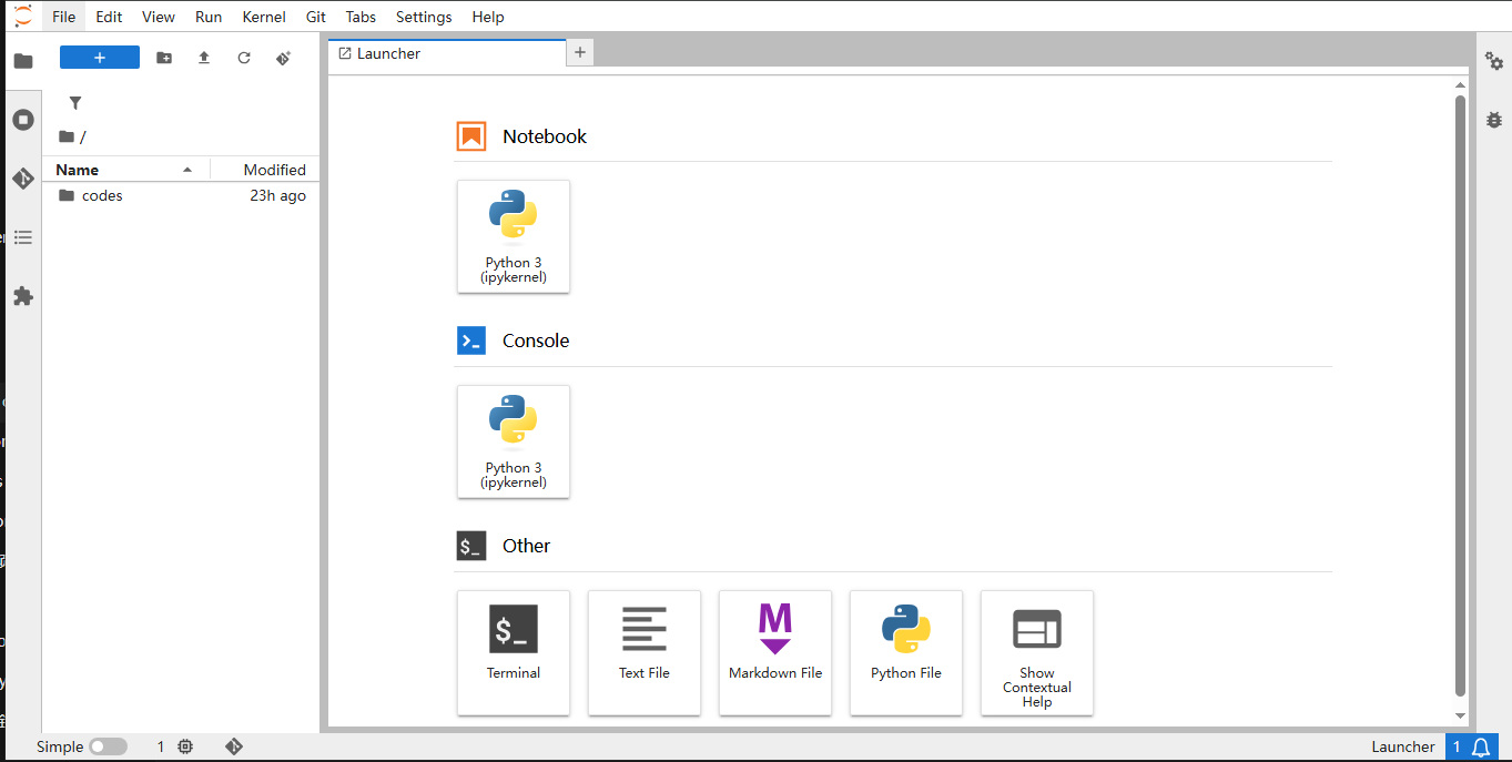
Figure 2 The interface of the login to the concise student version of ProtoPNet

Double-click the codes directory to see the ProtoPNet project directory (Figure 3).

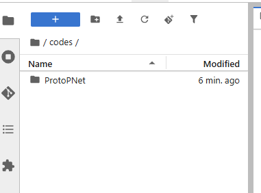
Figure 3 The engineering directory of ProtoPNet

Continue to double-click to enter the ProtoPNet directory, and you can see a number of subdirectories and files (Figure 4).

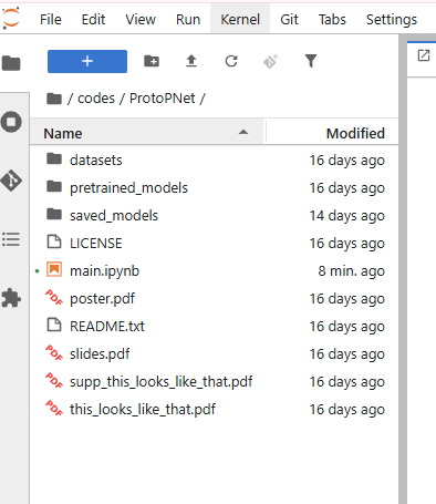
Figure 4 Subdirectories and files under the ProtoPNet directory

where,

• datasets, pretrained_models and saved_models are pre-prepared training and test data sets, pretraining models, and temporary storage files. They can be ignored at this time.

• LICENSE is an MIT license

• poster.pdf, slides.pdf, supp_this_looks_like_that.pdf and this_looks_like_that.pdf: They are the papers on the prototype part network (ProtoPNet) implemented in the original warehouse.

• main.ipynb - That’s the focus of this article.

This is the experimental version of the simplified ProtoPNet. It uses Jupyter Notebook as the runtime environment, with all required Python libraries and packages pre-configured in the cloud. Readers can simply open this main.ipynb online to read the code, set breakpoints, run and debug, view the intermediate variables, validate ideas, and compare algorithm details with those in the original paper.

Before we begin reading the code, let’s introduce how to use the debugging function of jupyter Notebook debugger to set breakpoints and observe the results of intermediate variables.

Double-click open main.ipynb, and then click to open the Debugger icon on the right (Figure 5):

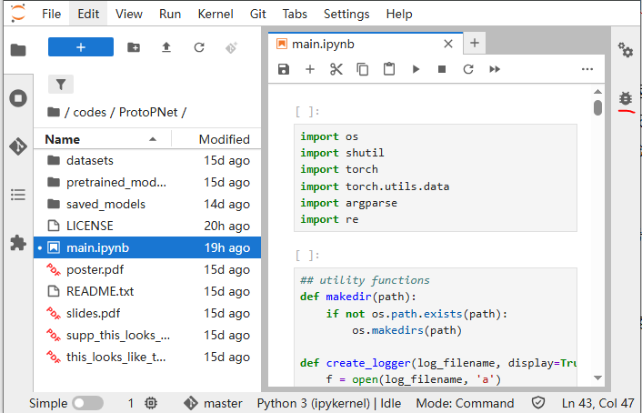
Figure 5 Open the debugger

Then find the Enable Debugger icon in the middle and right (Figure 6) and click it; wait until the icon turns red, indicating that the ‘Enable Debugger’ has been enabled successfully (Figure 7).

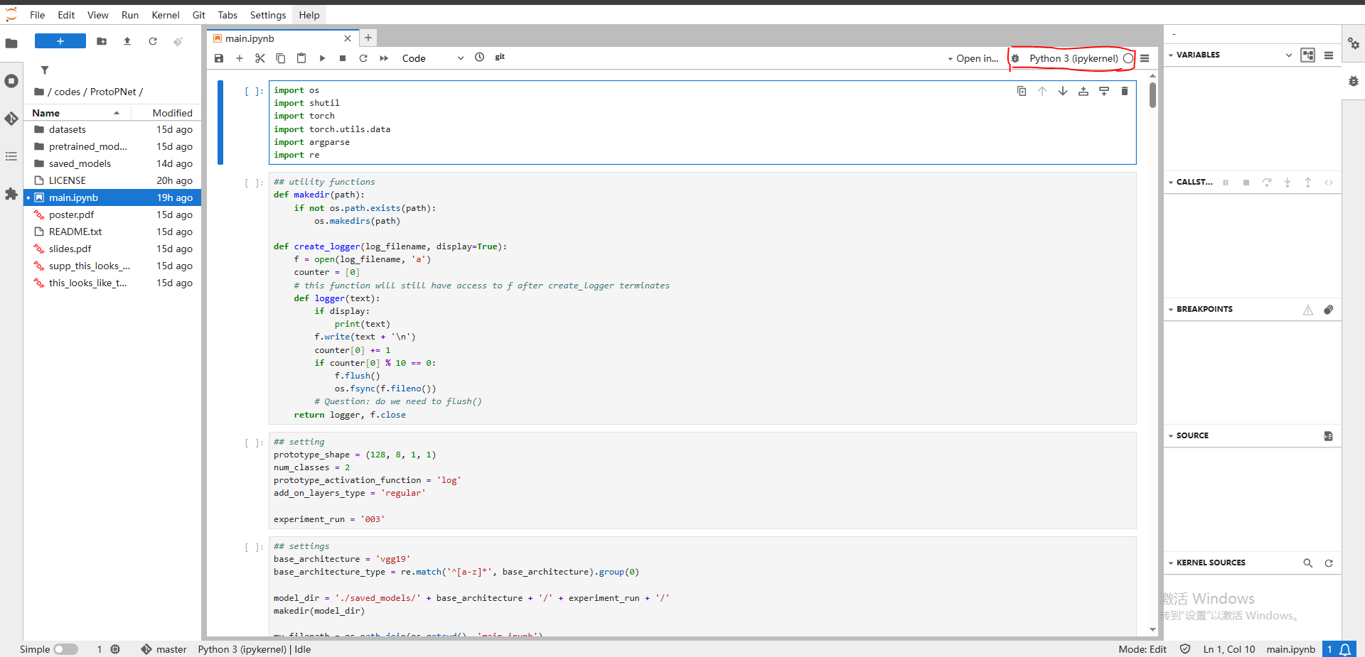
Figure 6 Click the Enable Debugger icon

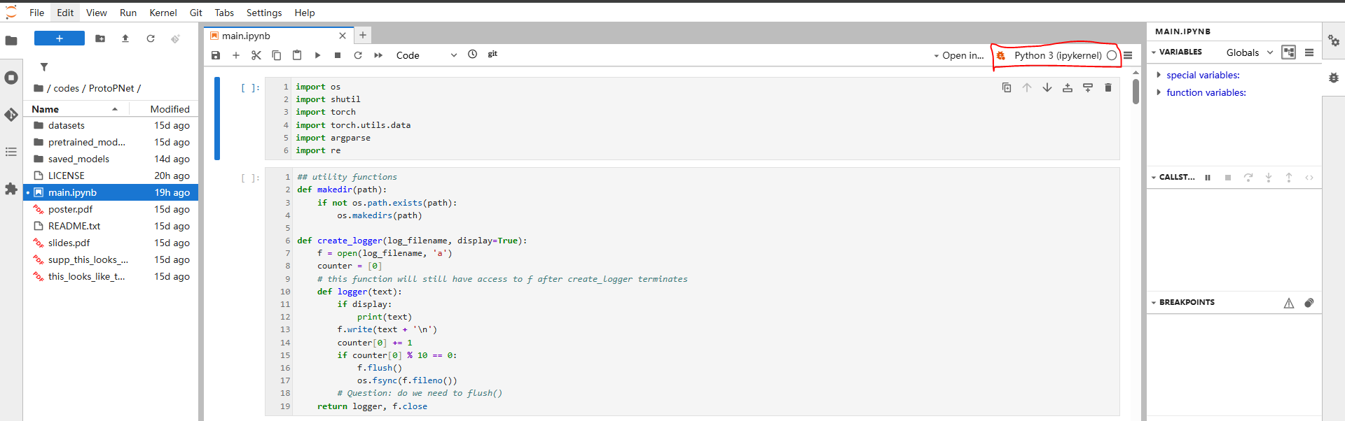
Figure 7 Icon status after successful Enable Debugger

Then click at the beginning of the first row in main.ipynb to add the first breakpoint (see Figure 8):

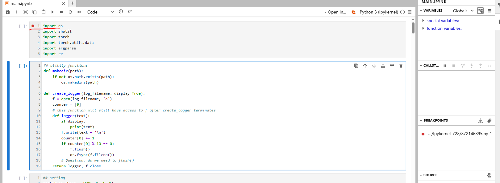
Figure 8 sets a breakpoint in the first row

Click the right triangle icon shown in Figure 9 to run the first cell of the notebook and wait for the background of the first line to turn gray, indicating that the program has reached the breakpoint at the first line.

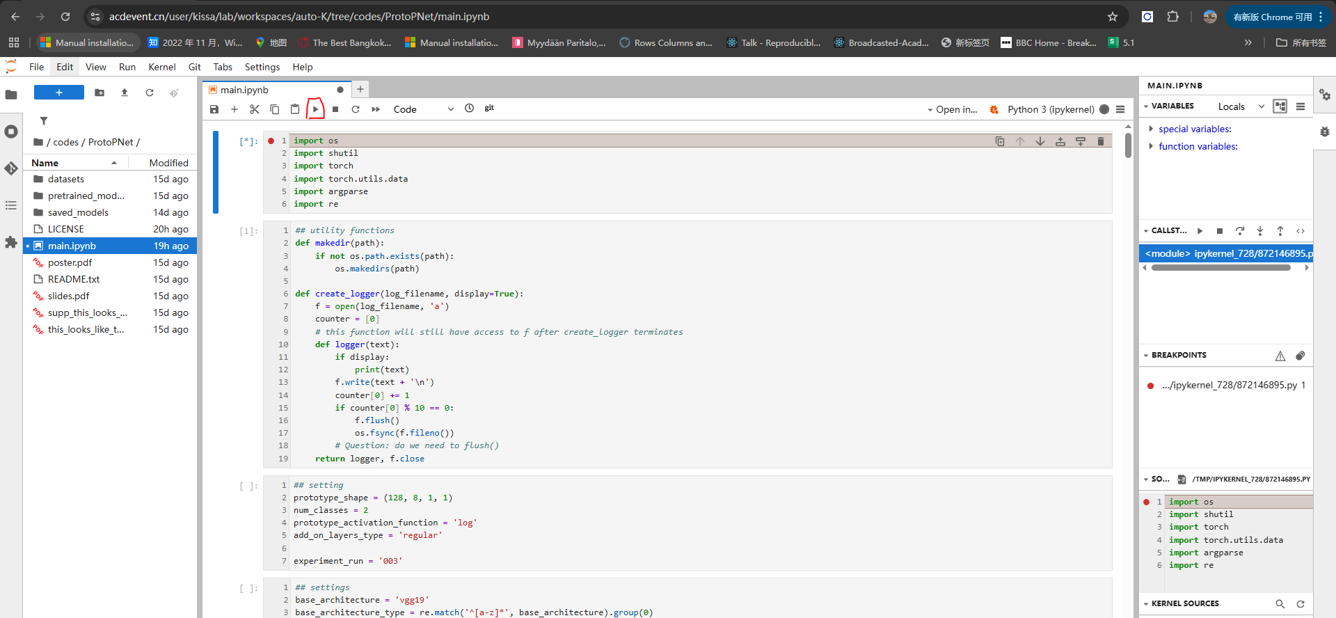
Figure 9 A unit selected for operation

Then, in the debugger window on the right, you can select Continue, Terminate, Next, Step In, Step-Out to debug; and Evaluate Code to calculate and print intermediate results (Figure 10).

Figure 10 choose to continue, terminate, next, enter the function, exit the function, execute the expression, etc

Here, select Terminate to end this debugging session and double-click the first line to cancel the breakpoint on that line (Figure 11).

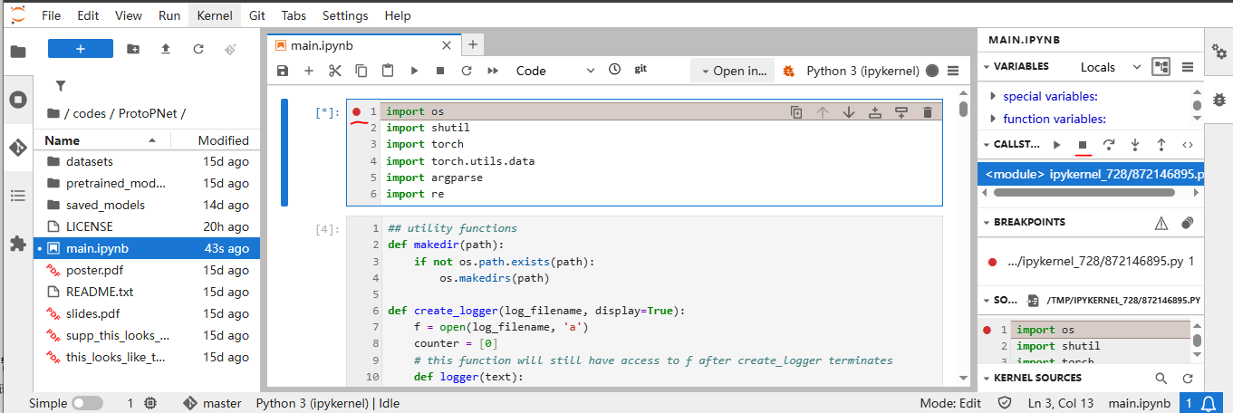
Figure 11 Selects to terminate debugging and cancel breakpoints

Then go to the eighth unit of main.ipynb and click on the ‘def forward (self, x)’ function in the first line of this function to add a new breakpoint (as shown in Figure 12):

Figure 12 Add a new breakpoint

Then select ‘Run→Run All Cells’ from the notebook menu (Figure 13) to run main.ipynb from scratch.

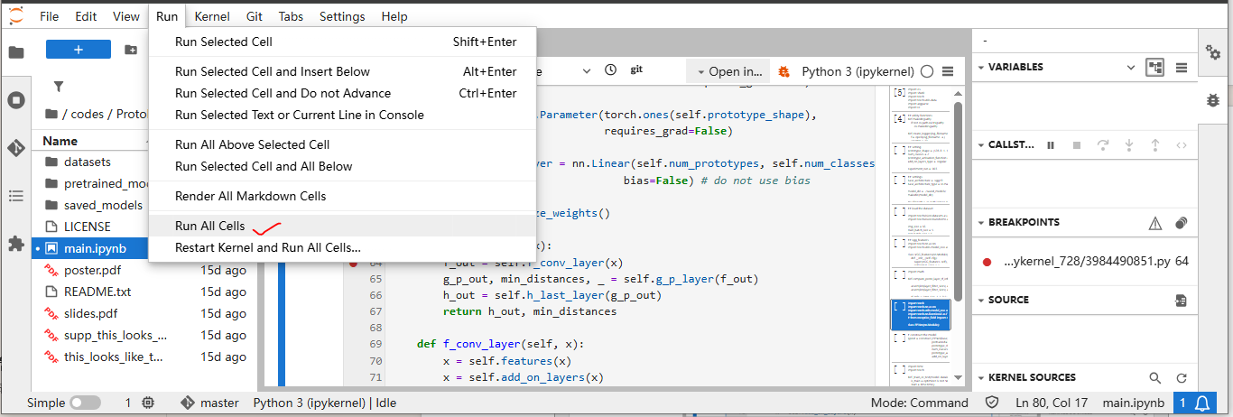
Figure 13 Select Run All Cells

If everything is normal, the program will pause at the breakpoint just set (Figure 14):

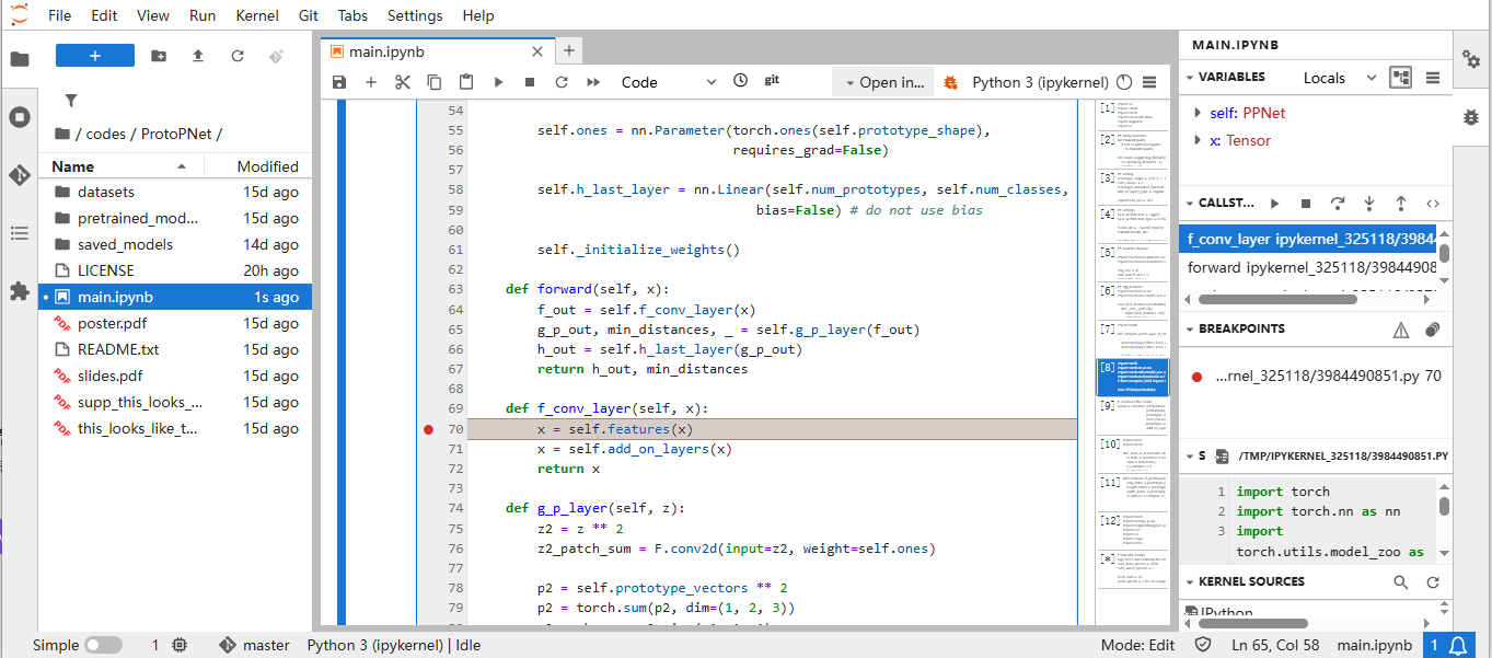
Figure 14 Pause at the new breakpoint

Then you can view VARIABLES, CALLSTACKs, etc. in the debugger window (Figure 15)

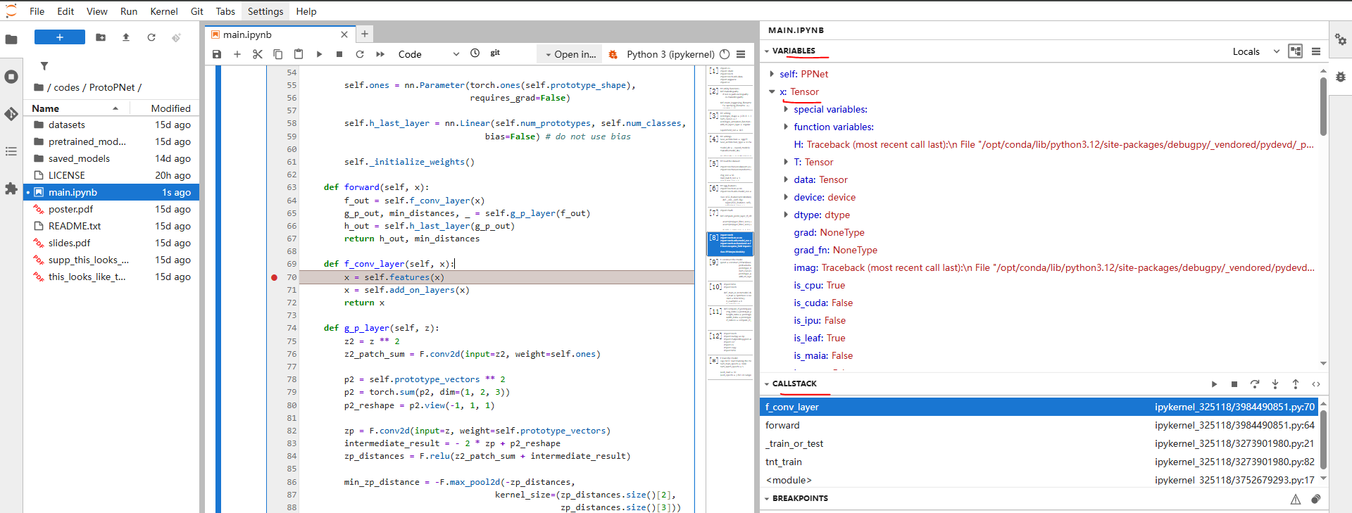
Figure 15. View variables, call stack, etc. in the debugger window

You can also use the “Evaluate Code” in the CALLSTACKs in Figure 16 and Figure 17 to print the value of a variable (such as Tensor x):

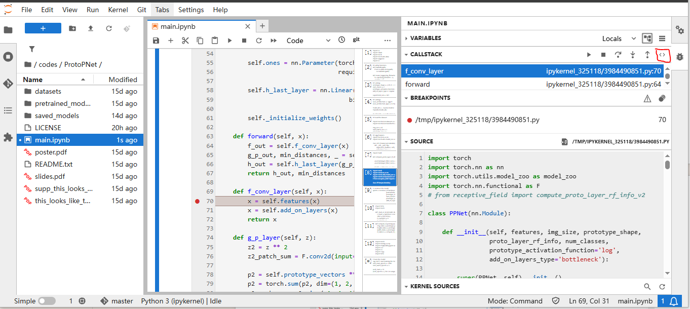
Figure 16. Example of using Evaluation Code-1

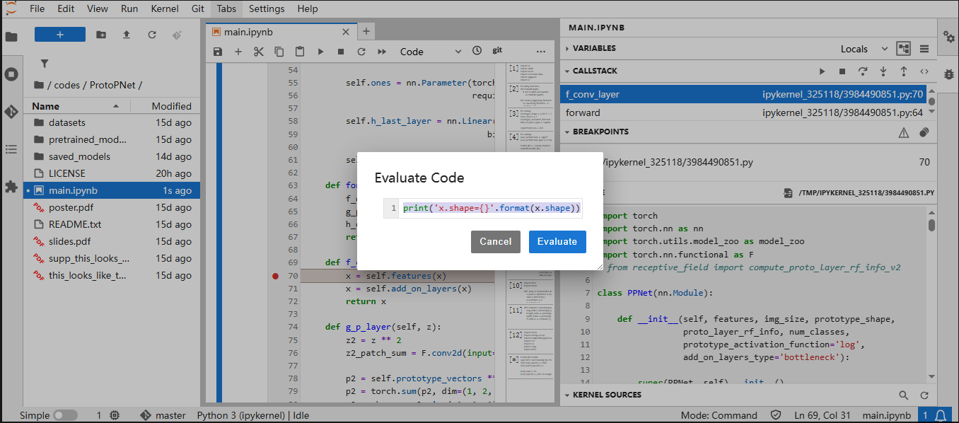
Figure 17. Example of using the Evaluation Code-2

The results of the print are displayed at the end of main.ipynb (Figure 18):

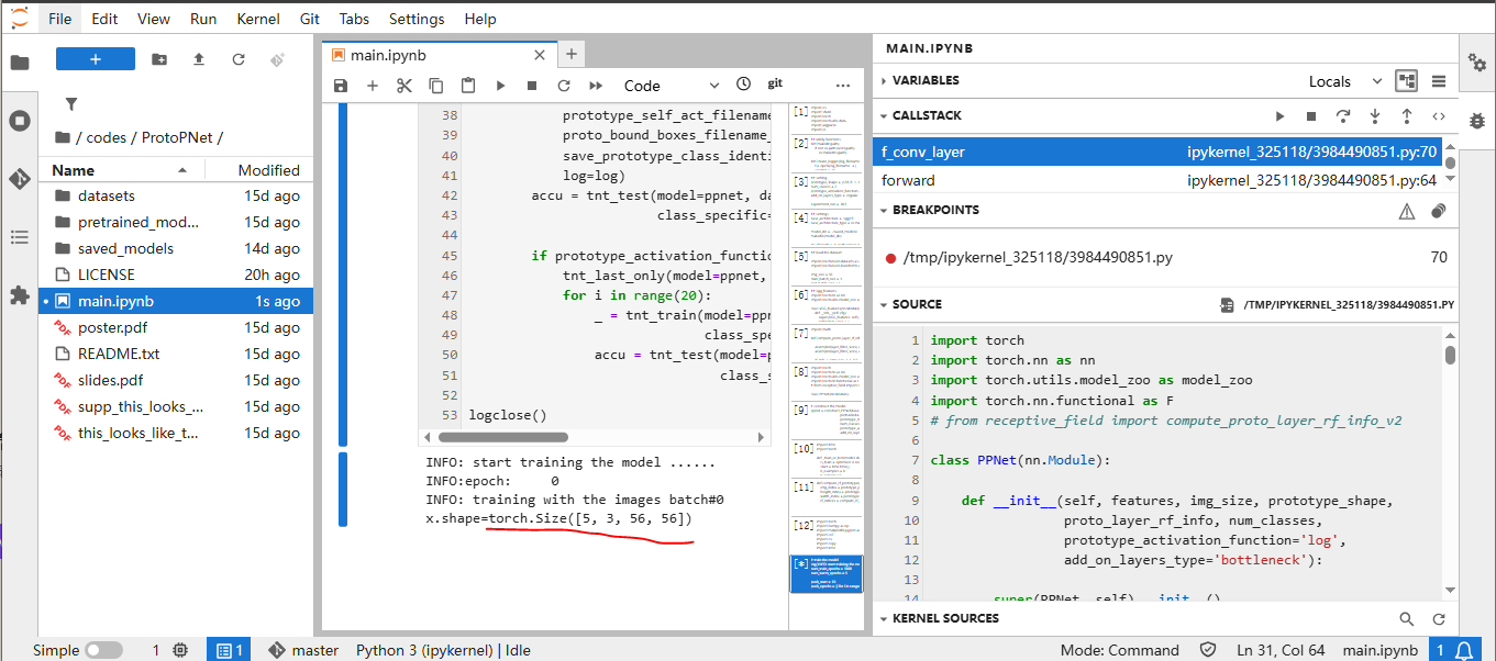
Figure 18 Check the output of Evaluation Code

If there is a problem with the above operation, such as “the program does not respond after clicking the run button for some time”, you can restart the kernel (as shown in Figure 19) and click the ‘run’ button again

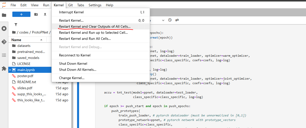
Figure 19 Restart kernel

This is the end of the first lecture. The next lecture will explain the algorithm principles of the paper, and compare it with the code and cross verify.

References

1. The original complete warehouse of ProtoPNet https://github.com/cfchen-duke/ProtoPNet

2. Academic Simulation Hub from AcdEvent.com, https://acdevent.com/simulation.html